For many applications in telemedicine or in a security context a contactless heart rate measurement can be great interest useful. Most of the conventional approaches use a wearable object like a chest belt or a special watch. In the mentioned cases, this is not always applicable. Therefore one is interested in methods, that can extract the heart rate from a video feed.
This project was part of the Computer Vision introduction course at École Polytechnique and is mainly based on this article
The basic idea behind will be, that when our heart is pumping, our skin is changing. We will detact these changes.

The first step for us was to use a face recognition system to extract the face from the video feed. For that, we used a Haar Cascade classifier in open CV to detect the face. The link for it can be found here.
What we do in the code is, to take an image or a series of images, that we will then further analyze. In the code, this can be done like that
import numpy as np
import cv2
import  face_detection
import  rate_compute
from scipy import ndimage

def main(framerate = 20, scale=0.1):
    """
    Input: The framerate in FPS and the scale of the video window
    Output: The video feed from the webcam
    """
    frame_buffer_object = []
    #here choose the video input source
    cap = cv2.VideoCapture(0)
    #cap = cv2.VideoCapture('./video/testing.mp4')
    while True:
        ret, frame = cap.read()
        coordinates = face_detection.detact_and_draw_box(frame, False)
        [...]
In the face detection method, we use the Haar-Cascade classifier. The code for this function is given by
import cv2 as cv2
import numpy as np
from skimage import io
import pdb
from matplotlib import pyplot as plt
#only works well for people without masks
face_cascade = cv2.CascadeClassifier('haarcascade_frontalface_default.xml')

def detact_and_draw_box(frame, drawing):
    """
    Input: A frame
    Output: The frame with bounding box on the face, only the largest one.
    """
    gray = cv2.cvtColor(frame, cv2.COLOR_BGR2GRAY)

    faces = face_cascade.detectMultiScale(gray, 1.1, 4)
    max = 0
    coords = (0,0,0,0)
    for (x, y, w, h) in faces:
        #only draw the one with maximal area. the others are probably noise.
        if(w*h>max):
            coords = (x, y, w, h)
            max = w*h

    coords = (x, y, w, h)
    if drawing==True:
        cv2.rectangle(frame, (x, y), (x+w, y+h), (0, 255, 0), thickness=2)
    return coords
This code mainly draws a rectangle on the frame as a face bounding box and returns the coordinates of the rectangle.
In the first part of the implementation, in order to get a region of interest of the forehead, we just used basic face proportion rules that one can use to cut out a rectangular part of the forehead. The implementation for such a method, to cut out the forehead can be done like that
def forehead_detection(frame, coordinates):
   """
   Input: A Frame and coordinates
   Output: A sliced frame, that only contains the forehead.
   """
   start_x = coordinates[0] + int(1/4*coordinates[2])
   stop_x = coordinates[0] + int(3/4*coordinates[2])
   start_y = coordinates[1] + int(1/20*coordinates[3])
   stop_y= coordinates[1] + int(1/6*coordinates[3])
   cv2.rectangle(frame, (start_x, start_y), (stop_x, stop_y), (0, 255, 0), thickness=2)

   #cut this part out then, then return it to analyse further.
   frame_mod = frame[start_y:stop_y,start_x:stop_x]
   return (frame,frame_mod)
In the values are a bit empirical, but nevertheless they provide a region in the face, that could look like that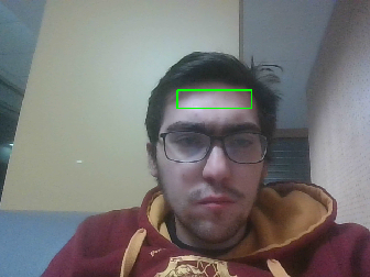
The function forehead_detection(frame, coordinates) returns the cropped region of interest, that only contains the forehead. This can then further be analyzed.
If one wants to use real time analysis, it is useful to use this segmentation method, because it is extremely quick. If one is more interested in a better region of interest, it is benefitial to use another segmentation method, such as a grab cut segmentation. In this case, the face can be extracted like that

The code, that mainly uses the openCv grab cut method, can be excecuted like that:
    def face_segmentation(frame, coordinates):
        mask = np.zeros(frame.shape[:2],np.uint8)
        bgdModel = np.zeros((1,65),np.float64)
        fgdModel = np.zeros((1,65),np.float64)
        rect = np.array(coordinates)
        #this is necessary to augment the size of the bounding box in order to fill in the whole face in a
        #rectangle, that we can pass to the graph cut segmentation function.
        rect[1] =int(0.5*rect[1])
        rect[3] = int(rect[3]*1.6)

        cv2.grabCut(frame,mask,rect,bgdModel,fgdModel,5,cv2.GC_INIT_WITH_RECT)
        mask2 = np.where((mask==2)|(mask==0),0,1).astype('uint8')
        graph_face = frame * mask2[:,:,np.newaxis]
        return(frame, graph_face)
In this case the entire cutted face is returned and can be used for further investigation.
The main method now has for a video with framerate of 30 fps a form like that
def main(framerate = 20, scale=0.1):
    """
    Input: The framerate in FPS and the scale of the video window
    Output: The video feed from the webcam
    """
    [...]
    while True:
        [ ...]
            fr, forehead = face_detection.face_segmentation(frame, coordinates)

            frame_buffer_object.append(forehead)
        if(len(frame_buffer_object)==(framerate)*30):
            frame_buffer_object.pop(0)
            rate_compute.detect_change(frame_buffer_object, 1/framerate, counter)
        cv2.namedWindow('Input',cv2.WINDOW_NORMAL)
        #cv2.resizeWindow('Input', 500,500)
        cv2.imshow('Input', forehead)
The purpose of this structure is to ensure, that at each time step we have the faces of a 30 second time window, such that we can compute the frequency spectrum in this time frame. For our purpose we assume, that the heart rate is constant in a 30 second time frame.
If we have the frame buffer over a 30 second time window, we can start to analyze it and fill the function rate_compute.detect_change(...) with content
Frequency analysis
After taking a ROI for each frame, we calculate the average values for RGB color channels of the ROI, denoted as $$x_R(t), x_G(t), x_B(t)$$ where t is the time. Then we use independent component analysis (ICA) to extract the source signals from the observed mixed color signals. The ICA is defined as follows: The data is represented by the observed random vector $$x = (x_1,\ldots, x_m)^T$$ and the hidden components as the random vector $$ s = (s_1,\ldots , s_n)^T .$$ The task is to transform the observed data $x$ , using a linear static transformation $W$ as $s = W x$, into a vector of maximally independent components $s$ measured by some function $$F(s_1,\ldots , s_n)$$ of independence. We use ICA by assuming that the source color signals are potentially non-Gaussian signals and that they are statistically independent from each other. Although this assumption might not be true if we consider the changes of blood volume and light intensity, but for a time window less then one minute, it is a reasonable approximation. The transformation in the ICA is linear, so the number of source signals is no more than the number of observed signals, and we assume there are three source signals $s_R(t), s_G (t), s_B(t)$ contributing to the observed color changes in the three channels. According to the definition of ICA, we have $$s(t) = W^{−1} x(t)$$ where $$x(t) = [x_R(t), x_G (t), x_B(t)]^T , s(t) = [s_1(t), s_2(t), s_3(t)]^T$$ and $W$ is a 3 × 3 linear transformation (matrix). We used an implemented FastICA function in the scikit-learn library to recover the approximate source signals $s(t)$. After extraction of the source signals $s(t)$, we can transform the signals on time into signals on temporal frequency using Fourier Transformation. The measured heart rate will be the frequency with highest magnitude in the range from 0.75 to 3 Hz, which corresponds to physiological heart rate ranges from 45 to 180 bpm.
You can think of the ICA as a technique, that can seperate from a signal with several sources the individual signals. For example in this journal
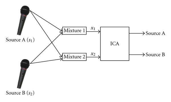
they illustrate this with the example, to extract one voice in a crowded room with several voices.
To implement the ideas explained above
def detect_change(buffer_object,Ts, counter_end):
    """
    Input: buffer object, a sequence of frames, The size of the time step and the
    Output: Either a plot of the heart rate over a 5 second time window
    """

    #print("enter detect_change")
    min_y = buffer_object[0].shape[0]
    min_x = buffer_object[0].shape[1]
    for j in range(len(buffer_object)):
        #if the programm failed to generate a
        if(buffer_object[j].shape[0]==0):
            buffer_object[j] = buffer_object[j-1]
        else:
            if(buffer_object[j].shape[1]<min_x):
                min_x = buffer_object[j].shape[1]
            if(buffer_object[j].shape[0]<min_y):
                min_y = buffer_object[j].shape[0]


    for idx in range(len(buffer_object)):
        #cut the pictures in the right size
        buffer_object[idx] = buffer_object[idx][:min_y,:min_x,::]
    buffer_np = np.array(buffer_object)
    red_channel = buffer_np[:,:,:,0]
    green_channel = buffer_np[:,:,:,1]
    blue_channel = buffer_np[:,:,:,2]
    [...]
We extract the channel values for the frame buffer object
def detect_change(buffer_object,Ts, counter_end):
    """
    Input: buffer object, a sequence of frames, The size of the time step and the
    Output: Either a plot of the heart rate over a 5 second time window
    """
    [...]
    #compute the mean per image to get an array that corresponds to the
    x_red = red_channel.mean(axis=(1,2))
    x_green = green_channel.mean(axis=(1,2))
    x_blue = blue_channel.mean(axis=(1,2))
    #normalize the signal over the entire time, i.e we will create a signal with zero mean and unit variance.
    mean_red = np.mean(x_red, axis=0)
    mean_green = np.mean(x_green, axis=0)
    mean_blue = np.mean(x_blue, axis=0)

    std_red = np.std(x_red, axis=0)
    std_green = np.std(x_green, axis=0)
    std_blue = np.std(x_blue, axis=0)

    x_red =  (x_red-mean_red)/std_red
    x_green =  (x_green-mean_green)/std_green
    x_blue =  (x_blue-mean_blue)/std_blue

    X_ = np.vstack((x_red,x_green,x_blue)).T

    transformer = FastICA(n_components=3, random_state = 0)
    S_ = transformer.fit_transform(X_)
    [...]
This gives us a signal, where we take at each frame the mean value of the color and extract the source of interest through the ICA. The assumption is, that when our heart is pumping, the color in the face is changing too. When we measure the frequency of this change of color, we want to deduce the heart rate from it.
Now we can apply the Fourier transformation to the extracted signals.
def detect_change(buffer_object,Ts, counter_end):
    """
    Input: buffer object, a sequence of frames, The size of the time step and the
    Output: Either a plot of the heart rate over a 5 second time window
    """
    [...]
    t = np.arange(S_.shape[0])
    red_fft = np.abs(np.fft.fft(S_[:,0]))**2
    red_freq = np.fft.fftfreq(np.size(S_[:,0],0),Ts)

    #extract with the mask only the values that are in the reasonable domain for the heart rate.
    indexing = np.ma.masked_where(np.abs(red_freq)<high_freq, red_freq)
    #indexing = np.ma.masked_where(True, red_freq)
    vals_to_keep = indexing.mask
    red_freq = red_freq[vals_to_keep]
    red_fft = red_fft[vals_to_keep]

    indexing = np.ma.masked_where(red_freq>low_freq, red_freq)
    #indexing = np.ma.masked_where(True, red_freq)
    vals_to_keep = indexing.mask
    red_freq = red_freq[vals_to_keep]
    red_fft = red_fft[vals_to_keep]
    [...]
We empirically deduce frequencies, that are too high and too low, which would be unreasonable. In this code snipped, we do this for the red values, but similarly, this can be done for the green and blue color channel. If we plot the data of the frequency spectrum in real time with the following code
    #pdb.set_trace()
    if plt_all_freq:
    #print('red_freq',red_freq)
        plt.clf()
        plt.title("frequency spectrum")
        plt.xlabel("x axis frequency")
        plt.ylabel("t axis value")
        plt.plot(red_freq, np.real(red_fft), color="red")
        plt.plot(green_freq, np.real(green_fft), color = "green")
        plt.plot(blue_freq, np.real(blue_fft), color = "blue")

        plt.draw()
        plt.pause(0.01)
we obtain the following plot
In this plot we need to focus on the first peak of the frequency, more precisely on the position of the peak. The position corresponds to the frequency. Here we still see the noisy data, where we have not cut of all the values below 0.75Hz, which would mean to have a heart rate of 45bpm. If we focus on the peak with frequency higher then 0.75, we get the heart rate. In practise it turned out, that it can be useful to take the mean of the red, green a blue heart rate for us. In this case we achieved for a stable sitting person values that were 5-10 bpm away from the ground truth, which we measured with a real heart rate sensor.
I took a video capture of myself during the 2021 Formula 1 season final.
In this case I took the mean of the heart rates obtained from the different color channels.
In general one can say, that if the lightning is uniform and one is not turning the head too much, the method yields values that are acceptable. Nevertheless, there are some severe failure cases. If a person is wearing Make-Up -for example for a TV interview- it is more difficult to detect the changes in the skin color through the heart pumping.
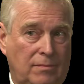
We tried our method on publicly available interviews, like the interview of Prince Andrew. But we found with our method, that he would have had a heart rate of 51bpm, which seems a bit unlikely.
The code for this project can be found under https://github.com/JeansLli/X-INF573-heart-rater.