In this TP we want to calculate the harmonic and the conformal parametrization of a mesh.
You will need to complete the class methods in the class ConformalParametrization that you will find in the file conformal.cpp. In order to see the goal of the TP, you can press 4 to use the pre-build Libigl method of the conformal parametrization on the mesh.
Minimizing the Dirichlet Energy and Harmonic Parametrization
In the first part of the TD it will be our objective to construct a parametrization that minimizes the Dirichlet energy. This energy will be also needed later on to calculate the conformal energy, which you will minimize for the conformal parametrization. The scenario will be that we prescribe in 2D a boundary curve and we will subsequently calculate for every vertex a 2D coordinate inside the bounded domain such that the Dirichlet energy is minimized.
As you have seen in the lecture, a function $u$ is a minimizer of the Dirichlet energy if and only if it is harmonic, i.e $$\mathrm{min}_{u}\ E_D(u) = \int_C |{\nabla u}|^2 \Leftrightarrow \Delta u = -\Delta u = 0.$$
To compute the minimization of this energy, and with it the surface parametrization, we will solve the Poisson problem with a constraint on the boundary, i.e we want to solve. $$-\Delta u = 0,\quad\text{where }\quad u\mid_{\partial M} = u_{\text{boundary constraint}}$$
As a first step you should build the matrix for the laplacian. To do that complete the method compute_dirichlet() in the class ConformalParametrization to build the discrete Laplacian as a sparse matrix (see below).
Remark: The equation you are solving in here is a Poisson problem of the form $$ -\Delta u = 0.$$ If you compare this with the heat equation $$\partial_t u = \Delta u,$$ these are two equations, that involve the Laplacian. In the continuous case, this is exactly the same operator. However in the discrete case it makes a difference, whether we regard the Laplacian as a pointwise or an integrated quantity. From a mathematical point of view it is equivalent to solve $$-\Delta u = -A^{-1} L u = 0$$ or $$-Lu = A\cdot 0 = 0.$$ However from a numerical perspective it is benificial to consider systems that involve symmetric, positive definite matrices, sin ce it is easier to solve them and allows to use tailored minimizers.
Therefore, in contrast to the operator in the previous exercise, you do not need to calculate the Voronoi areas. It is sufficient to compute the matrix $L$. We recommend you to debug your build with the provided hexagon, where you can by hand check the cotangent weights. Make sure that the matrix $-L$ is indeed positive definite!
Sparse Matrices in Eigen
The matrices of interest will be sparse in our case. Therefore we are using a different datastructure to represent these matrices. Instead of saving every matrix entry, we will only save the non-zero entries with their respective positions and the value of the matrix at this entry.
A sparse matrix with double values can be declared through Eigen::SparseMatrix<double>. In order to create such a matrix we need to create Triplets
Eigen::Triplet<double>(row, column, value) and stack them in a vector. Then we can use the method setFromTriplets to fill the sparse matrix. We will need matrices of this type to use the in-build solver.
Once the matrix $L$ is calculated, you can compute the harmonic parametrization. To do this, complete the method compute_harmonic_parametrization(MatrixXd &V_uv_harmonic). To do that you should first determine the boundary vertices of your mesh. You can use the provided method igl::boundary_loop() to do that. Next, you need to set a 2-d boundary shape so that you map every boundary vertex to a determined point in the plane.
We recommend to use the camelhead as a shape, since you will need to parametrize only one boundary in this case.
To calculate the minimizer in your method compute_harmonic_parametrization(MatrixXd &V_uv_harmonic) you can now make use of an in-build solver for constrained minimization problems.
Minimization of quadratic energies in Libigl
To calculate the minimizer of quadratic energies under constraints, Libigl has an in-build method to solve these kind of quadratic minimization problems. For a general sparse, symmetric, positive definite $n\times n$ matrix $Q$ (hint: check whether your matrix is really positive definite…) and a vector $B$, let $\mid \text{Constraints} \mid$ be the number of constraints for the minimization. Let $z_{\partial M}$ be a vector of shape $\mid\text{Constraints} \mid\times 1$ (Attention: not $\mid \text{Constraints} \mid\times 2$ !!) that indicate the where a constraint is set. Let $z_{bc}$ be a vector of shape $\mid \text{Constraints} \mid\times 1$ encoding the constraints for the chosen points. In our cases for this task we can set $A_{eq} = 0$, an empty sparse matrix and $B, B_{eq}$ as zero vectors. Then we can solve the minimization problem $$\mathrm{min}_z \ z^t Q z + z^t B,\quad \mathrm{where}\quad z_{\partial M} = z_{bc}\quad \mathrm{and}\quad A_{eq}\ z = B_{eq} \qquad(1)$$ with the method
igl::min_quad_with_fixed_data<double> data;
igl::min_quad_with_fixed_precompute(Q, zb, SparseMatrix<double>(),true, data);
igl::min_quad_with_fixed_solve(data,B,zbc,VectorXd(),minimal_z);
Task:
Solve for the minimizer of the problem
$$\text{min}_z\ \ z^T (-L) z\quad \text{ where } \quad z_{\partial M} = z_{bc}$$
to compute the coordinates of the harmonic parametrization and overwrite the matrix V_uv_harmonic. Experiment with different boundary shapes.
Notational Remark: For the description of the smooth problem it is a common convention to use the letter $u$ as argument for the (smooth) Dirichlet energy. However for the description of the minimization of discrete quadratic energies, it is more common to use the letter $z$ as argument (especially the arguments in the code of the minimizer are named by default z).
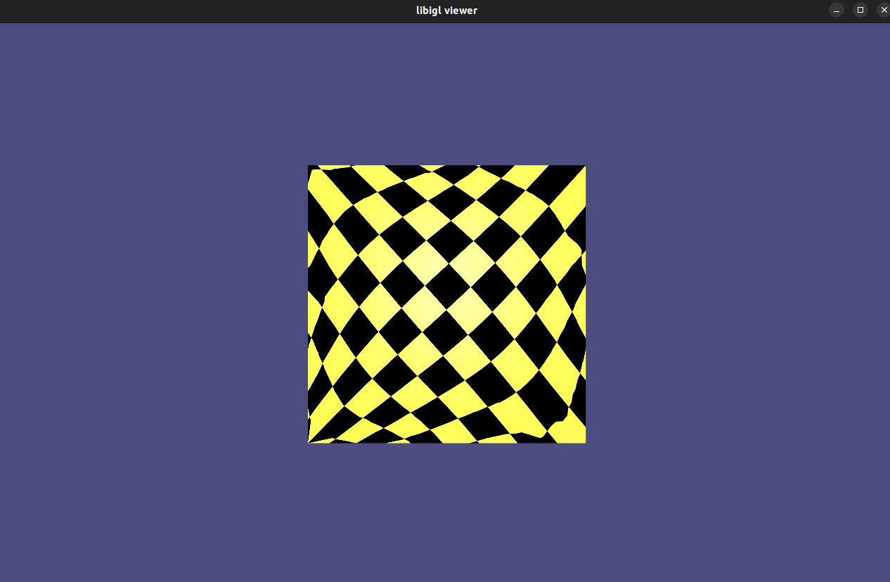
The harmonic parametrization of the camelhead, where each boundary vertex is mapped to a square could look like that.
Bonus:
Solve this problem without the in-build solver and code the constraint minimization yourself. Set up the Lagrange function $$\mathcal{L}(z,\lambda)$$ of the minimization problem under constraints $(1)$ and calculate the Lagrange multipliers $\lambda$. Transform the problem by a calculation on paper into a problem where a linear solve is sufficient to determine the parametrization. Attach a pdf of your calculation with explanation to your submission and implement this minimization.
Conformal Parametrization
With the working Dirichlet energy we can now focus on the minimization of the conformal energy to calculate a conformal parametrization.
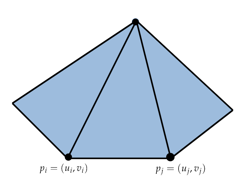
In order to do this, note that the area of a discrete mesh can be computed through $$\mathrm{Area}(M) = \sum_{e_{ij}\in \partial M}\frac{1}{2} (u_i v_j - u_j v_i),$$
From this you should build a matrix $A$ such that
$$\text{Area}(M) = \begin{pmatrix} u_1,v_1,u_2,v_2,\ldots,u_{|V|},v_{|V|}\end{pmatrix}\cdot A\cdot \begin{pmatrix} u_1,v_1,u_2,v_2,\ldots,u_{|V|},v_{|V|}\end{pmatrix}^T$$ Note: The way to arrange coordinates is not unique! In case you used a different order of coordinates to assemble the Laplacian, you need to be consistent with it.
Build a sparse matrix Area, complete the methods build_area with the formula from the lecture and build_conformal_energy.
With this matrix in place complete the method compute_conformal_energy and build the matrix $\mathrm{Conformal}$ such that
$$E_{\mathrm{Conformal}}(z) = z^T\ \cdot \mathrm{Conformal}\ \cdot z$$
In the case of the harmonic parametrization we set a constraint on every vertex on the boundary. To complete the method minimize_energy you will fix the positions of 2 vertices on the boundary. Then modify the constraint minimization of the dirichlet energy to calculate the minimizer of the conformal energy under the given constraint. From that calculate the coordinates of the conformal parametrization and overwrite the matrix V_uv.
Experiment with fixing different vertices on the boundary or to place them at different positions.
Bonus:
Until now we have used the Laplacian with cotangent weights. Now, try to use a Laplacian with different weights. For example, the euclidean distance between adjacent vertices or just the binary information (1 or 0) whether two vertices are connected. In the case of the combinatorial Laplacian, the weights are given through $$L_{ij} = \begin{cases} 1,\ \mathrm{if}\ (i,j)\in \mathcal{E}\ 0,\ \mathrm{if}\ (i,j)\notin \mathcal{E}\end{cases}\quad \mathrm{and}\quad L_{ii} = \sum_{(ij)\in\mathcal{E}} L_{ij}.$$ For the Laplacian that uses the euclidean distances, the weights are given through $$L_{ij} = \begin{cases} ||{v_i-v_j}||,\ \mathrm{if}\ (i,j)\in \mathcal{E}\ 0,\ \mathrm{if}\ (i,j)\notin \mathcal{E}\end{cases}\quad \mathrm{and}\quad L_{ii} = \sum_{(ij)\in\mathcal{E}} L_{ij},$$ thus you only have to make minimal changes for your sparse matrices.
However if you just change the Laplacian like that and try to build the conformal energy you might run in a numerical error. Why is that the case and what do you have to do to change that ?
Bonus:
Now that we have calculated the conformal parametrization of the mesh, you will realize that if you fix different points of the mesh as a constraint for the minimization, you will obtain different parametrizations.
The conformal parametrization is angle preserving, but not area preserving. Two triangles that have the same angles can be transformed through a scaling and a rotation into each other.
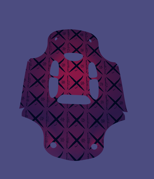
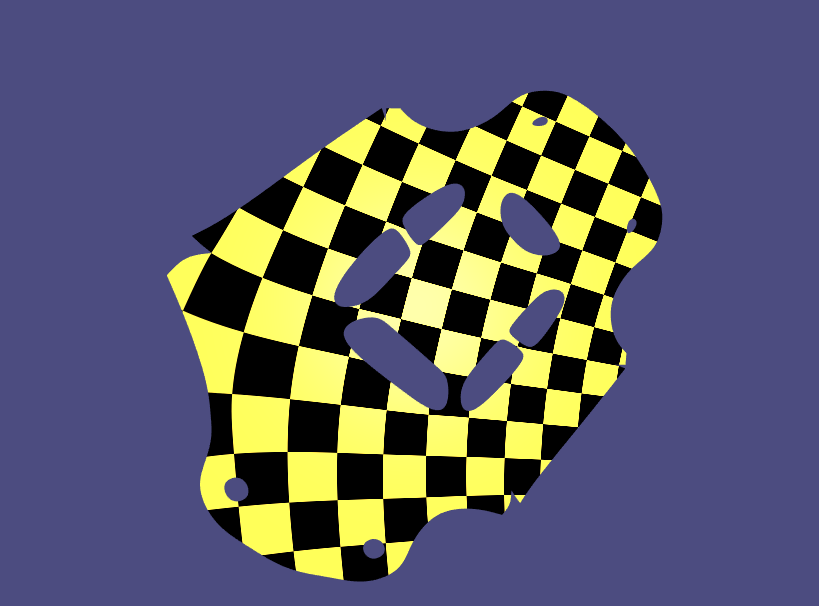
Your task is now to compute this scaling factor –the conformal factor– and color the parametrization with this factor. Fix different points of the mesh in the plane and compare the area distortion. Attach screenshots of the coloring of different meshes to your submission. Note that the conformal factor in the method compute_conformal_factor has to be computed per triangle. In order to obtain a coloring per vertex, you need to calculate subsequently the mean over the one ring neighborhood and determine a useful color scale in the method compute_conformal_coloring. Furthermore use the newly computed UV coordinates to map a texture onto the flattened mesh.